Jekyll2026-09-29T12:39:58+00:00https://kovashikawa.com/feed.xmlRafael KovashikawaData Scientist & AI Engineer at FUSE. Writing about AI agents, MCP servers, quantitative finance, and data engineering.{"name"=>nil, "avatar"=>"/assets/images/selfie-avatar.webp", "bio"=>"AI Engineer @ FUSE. Previously macro quant @ JGP. MIT MicroMasters. Washington, DC.", "location"=>"Washington DC", "email"=>nil, "links"=>[{"label"=>"Email", "icon"=>"fas fa-fw fa-envelope-square"}, {"label"=>"Website", "icon"=>"fas fa-fw fa-link"}, {"label"=>"Twitter", "icon"=>"fab fa-fw fa-twitter-square"}, {"label"=>"Facebook", "icon"=>"fab fa-fw fa-facebook-square"}, {"label"=>"GitHub", "icon"=>"fab fa-fw fa-github", "url"=>"https://github.com/kovashikawa"}, {"label"=>"LinkedIn", "icon"=>"fab fa-fw fa-linkedin", "url"=>"https://www.linkedin.com/in/rkovashikawa/"}]}Stack Overflow Is Selling Proof That a Human Wrote It2026-09-18T00:00:00+00:002026-09-18T00:00:00+00:00https://kovashikawa.com/ai/stack-overflow-proof-of-authorshipStack Overflow brought Developer Story back on September 10, four years after the
2022 shutdown. The announcement
is unusually blunt about why.
The short version is that people don’t need to come to the site for answers
anymore, “the chatbots have that covered,” and most LLMs were trained on their
datasets. So the goal is not winning back question traffic. It is evidence that a
specific human wrote a specific thing.
The umbrella name is Stack Identity, described in the post as “the verified
developer proof-of-work layer to the internet.” Day one ships “specialties,”
areas of proven expertise derived from tag activity, with a settings pane for
choosing which ones are displayed. Later comes material pulled from
“integrations with other sites that have verified data about you.”
Not a LinkedIn pivot
My first read was that this is Stack Overflow turning into LinkedIn. It isn’t.
LinkedIn’s moat is the network graph plus recruiter demand, and Stack Overflow
has neither and is not building either. This reads more like a notary. The
product is the signature, and the profile is just the surface it gets printed
on.
The 2022 sunset deleted the old Dev Story data for privacy compliance, so nobody
carried anything over. A notary with no back catalog has to sell a signature that
starts today. My own record is the illustration. Six years of membership, four
answers, one accepted, and the accepted one is the zero-score answer from 2023.
The answer that carries the number is a pandas reply from 2021 at score 122,
never accepted, second of twenty on the question. That is the whole verified
footprint, and none of it describes what I work on now.
Verification needs a second party
A signature only has value when someone else accepts it. “Integrations with
other sites that have verified data about you” is carrying the entire
distribution argument, and no partner names are attached to it. The hard part is
not the profile UI or the trust model. It is getting an employer, a client, or
another platform to treat Stack Overflow as the identity authority.
They also run agents.stackoverflow.com, a
separate site in beta where the users are AI agents. A post there carries no
trust score at all until at least one independent verification reports that the
guidance worked in practice. Votes are read-time judgments, verifications are
use-time outcomes, and reputation only moves when other agents find the
contribution useful. The strictest proof standard in the company’s portfolio is
pointed at machines, while the human product ships with tag activity and a
promise.
Both are bids to define what counts as proof of work. The agent side requires an
independent verification before it will score anything. The human side starts
with the tags you already answered.
]]>{"name"=>nil, "avatar"=>"/assets/images/selfie-avatar.webp", "bio"=>"AI Engineer @ FUSE. Previously macro quant @ JGP. MIT MicroMasters. Washington, DC.", "location"=>"Washington DC", "email"=>nil, "links"=>[{"label"=>"Email", "icon"=>"fas fa-fw fa-envelope-square"}, {"label"=>"Website", "icon"=>"fas fa-fw fa-link"}, {"label"=>"Twitter", "icon"=>"fab fa-fw fa-twitter-square"}, {"label"=>"Facebook", "icon"=>"fab fa-fw fa-facebook-square"}, {"label"=>"GitHub", "icon"=>"fab fa-fw fa-github", "url"=>"https://github.com/kovashikawa"}, {"label"=>"LinkedIn", "icon"=>"fab fa-fw fa-linkedin", "url"=>"https://www.linkedin.com/in/rkovashikawa/"}]}Beyond Correlation: measuring dependence the modern way2026-09-02T16:00:00+00:002026-09-02T16:00:00+00:00https://kovashikawa.com/statistics/beyond-pearsons-rhoPearson’s correlation is zero for plenty of pairs that are fully dependent. The canonical case: $X \sim \mathcal{N}(0,1)$, $Y = \lvert X \rvert$. $\rho$ reports about 0, but $X$ determines $Y$ exactly. The fix isn’t “use a nonlinear measure” in the abstract, it’s knowing which measure catches which failure mode, and what each one actually guarantees.
That’s what this post benchmarks: distance correlation, Chatterjee’s xi, HSIC, KSG mutual information, and tail dependence, against nine synthetic datasets built to break Pearson in different ways.
Two minutes covering the same ground visually, walking through each counterexample and measure below.
The benchmark table
Measure
linear
quadratic
abs
sine
circle
cross
independent
heavy_tail
tail_t
Pearson
0.980
-0.017
-0.015
0.004
0.004
-0.028
0.000
0.729
0.484
Spearman
0.978
-0.014
-0.014
0.026
0.003
-0.010
0.004
0.795
0.477
Kendall
0.874
-0.011
-0.011
0.023
0.000
-0.007
0.003
0.614
0.343
Chatterjee xi
0.812
0.999
0.999
0.997
0.254
0.245
-0.004
0.449
0.164
Distance corr
0.971
0.543
0.559
0.253
0.197
0.313
0.014
0.768
0.468
HSIC
0.088
0.045
0.051
0.008
0.019
0.033
0.000
0.043
0.010
KSG MI
1.639
6.102
6.378
4.716
5.167
6.194
0.001
0.568
0.192
Tail dep (q=0.95)
0.856
0.498
0.498
0.090
0.000
0.462
0.032
0.500
0.376
n = 10,000, seed 42, full generator code in the repo.
The first three rows are the classical toolkit, and none of them catch quadratic, abs, sine, circle, or cross. Chatterjee’s xi, distance correlation, and KSG MI catch all five. HSIC and tail dependence are subtler cases, covered below. That gap is the whole problem, quantified.
Two things worth flagging before the per-measure sections.
Cross is the sharpest counterexample. $Y = X \cdot W$, where $W$ is a random sign independent of $X$. The sign cancels out any linear relationship, so Pearson, Spearman, and Kendall all read near zero. But $Y$ is not independent of $X$: $\lvert Y \rvert = \lvert X \rvert$ always. Chatterjee’s xi (0.245) and distance correlation (0.313) both catch it. Both margins are standard normal here, and the pair still isn’t jointly Gaussian, which is exactly the case where “uncorrelated implies independent” fails.
The measures split into two questions. Xi, distance correlation, HSIC, and KSG MI test dependence across the whole distribution. Tail dependence tests something narrower: whether extremes move together, which is why the tail_t column exists. HSIC is unnormalized and MI is measured in nats, so don’t compare magnitudes across measures. Use them to detect and rank, not to score.
The independent column is the null. Every measure should read near zero there, and does: Chatterjee’s xi is -0.004, distance correlation 0.014, HSIC 0.000. That’s the reference for judging every “catch” above. Xi’s null standard deviation is about $\sqrt{2/(5n)} \approx 0.0063$ at $n = 10{,}000$ (derived below), which puts circle’s xi of 0.254 roughly 40 null standard deviations out, not just “nonzero.”
Distance correlation
Szekely, Rizzo and Bakirov (2007) introduced distance correlation to fix exactly this blind spot. The idea: independence is equivalent to the joint characteristic function factoring into the product of marginals. Distance covariance is a weighted norm on exactly that difference, and the estimator falls out as a double-centering of pairwise distance matrices:
The property that matters: $\operatorname{dCor} = 0$ if and only if $X$ and $Y$ are independent, for distributions with finite first moments, in any dimension. Pearson cannot make that claim. In the bivariate normal case dCor is a deterministic function of $\lvert \rho \rvert$ and never exceeds it.
Cost: the naive estimator used here is $O(n^2)$ memory and time, because of the pairwise distance matrices. Fine at 10k rows, painful at 10M. Faster $O(n \log n)$ algorithms exist for univariate data (Huo and Szekely 2016).
Chatterjee’s rank correlation
Chatterjee (2021) took a different route, with a coefficient that is almost absurdly simple. Rank X, reorder Y’s max-ranks by X, and measure how much adjacent ranks jump:
where $r_i$ are the max-ranks of $Y$ reordered by $X$ and $g_i = (\text{max-rank of } -Y_i)/n$, so that $r_i/n$ and $g_i$ lie in $[0, 1]$. With no ties this collapses to $\xi = 1 - \frac{3}{n^2-1}\sum_{i=1}^{n-1}\lvert r_{i+1} - r_i \rvert$. For non-constant $Y$, the population coefficient $\xi$ satisfies: $\xi = 0$ iff independence, $\xi = 1$ iff $Y$ is a measurable function of $X$. Computes in $O(n \log n)$ and is completely nonparametric.
Three footnotes. First, under independence $\xi_n$ has mean zero and standard deviation about $\sqrt{2/(5n)}$, so it lands negative about half the time; that is expected, not a bug. Second, $\xi(X, Y)$ is asymmetric by construction: it measures “how well Y behaves as a function of X,” which the paper argues for deliberately. Third, xi has low power against many smooth alternatives (Shi, Drton and Han 2022), so treat a low xi as “no strong signal,” not “no dependence.”
HSIC
HSIC comes from the kernel methods literature (Gretton et al. 2005) and became a standard tool in nonlinear feature selection (Song et al. 2012). Map each variable into a reproducing kernel Hilbert space with a universal kernel (RBF here), and take the squared Hilbert-Schmidt norm of the cross-covariance operator between the two embeddings. HSIC = 0 iff independence for universal kernels (Gretton 2005 on compact domains; Fukumizu et al. 2008 for the general statement).
On this benchmark HSIC is the flattest row: 0.088 on linear, dropping to 0.008 on sine and 0.000 on independent, everything within a factor of about 11. It still separates dependent from independent, linear and heavy_tail sit well above the 0.000 null, but the RBF kernel’s median-distance bandwidth is not tuned per dataset here, so treat the exact HSIC values as a coarse detector rather than a ranking. Its real strength is scaling to vector-valued or high-dimensional X and Y, where density-based measures like KSG MI become impractical.
KSG mutual information
Mutual information $I(X; Y) = 0$ iff independence, full stop. The KSG estimator (Kraskov, Stogbauer and Grassberger 2004) is a k-nearest-neighbor scheme that adapts its resolution in both margins, which fixes the classic histogram-bin problems. It is what scikit-learn’s mutual_info_regression uses under the hood, with $k = 3$ neighbors here.
The values are not comparable across datasets. Linear has additive noise and a finite population MI of $-\frac{1}{2}\ln(1-\rho^2)$. At the generator’s $\rho \approx 0.9806$ that works out to about 1.629 nats, matching the 1.639 estimate. Quadratic, abs, sine, circle, and cross have no additive noise: each Y is fully determined by X and a coin flip or angle draw with no residual randomness, so the joint distribution is singular and the population MI is infinite. The KSG estimate for these just grows with $n$ and shrinks with $k$. So “6.4 nats on abs” does not mean abs is four times more dependent than linear’s 1.6. MI answers “is there dependence” decisively, and “how strong” only loosely.
The maximal information coefficient (Reshef et al. 2011) is the other mutual-information-based measure people reach for, maximizing normalized MI over grid binning schemes. It made a splash in Science in 2011, but its equitability claims were shown mathematically impossible for any nontrivial measure (Kinney and Atwal 2014), and later power comparisons found it underpowered relative to distance correlation (Simon and Tibshirani 2014). Refined variants followed (Reshef et al. 2016). Treat MIC, like the measures above, as a detector rather than a calibrated strength scale. It is not in this benchmark: minepy, the standard implementation, requires a compiled extension and was left out; the Reshef lab’s Java MINE tool is the reference implementation.
Tail dependence
The measures above test dependence across the whole distribution. Risk work cares about the tails specifically: given that one asset is above its 95th percentile, how likely is the other to be too? Tail dependence coefficients go back to Sibuya (1960); the modern treatment is Joe (1997).
The population quantity is the limit, if it exists:
The benchmark row reports the finite-quantile estimator $\lambda(q)$ at $q = 0.95$, a standard VaR level, exactly 500 conditioning exceedances at $n = 10{,}000$. Under independence, $\lambda(q) = 1 - q = 0.05$ exactly. The independent column reads 0.032, about 1.8 standard errors low (SE $\approx \sqrt{0.05 \cdot 0.95 / 500} \approx 0.0098$), consistent with the null.
This is where the Gaussian copula earns its infamy. For any correlation $\rho < 1$, the Gaussian copula has zero tail dependence in the limit, but the co-exceedance probability vanishes slowly as $q \to 1$. The linear column is generated from a Gaussian copula at $\rho \approx 0.9806$. Its finite-q estimator reads 0.856 at $q = 0.95$ against a closed form of 0.838. That gap narrows only gradually: about 0.74 by $q = 0.999$ and 0.70 by $q = 0.9999$. If your risk model is Gaussian-copula shaped and you feed it Pearson correlations, you are asserting away joint tail risk by construction, just with a delay.
The tail_t column is the counterexample. It’s generated from a $t$-copula with $\nu = 3, \rho = 0.5$, which has positive asymptotic tail dependence: $\lambda_U = 2T_4(-\sqrt{4/3}) \approx 0.31$. The empirical estimate at $q = 0.95$ reads 0.376, higher than the asymptotic limit because finite-q estimates overstate $\lambda_U$ and converge to it slowly, the same effect visible in the linear column above.
The heavy_tail column is a warning about reading too much into a name. It’s just $X$ plus independent $t_3$ noise, which is asymptotically tail independent despite the heavy-tailed marginal. Larger simulations ($n = 20$M) show its $\lambda(q)$ decaying with $q$: 0.487 at $q = 0.95$, 0.011 at $q = 0.999$, below 0.001 at $q = 0.9999$. The 0.500 in the benchmark table is the $n = 10{,}000$ estimate at $q = 0.95$ only, consistent with the larger simulation’s first point; the decay only shows up once $q$ moves well past 0.95. Always check the generator, not the label.
When to use what
Bivariate, monotone, want a sign: Spearman or Kendall.
Bivariate, any shape, want a [0, 1] strength: distance correlation or Chatterjee xi.
High-dimensional or vector-valued: distance correlation, HSIC.
Nonlinear feature screening: HSIC, KSG MI.
Portfolio and risk: tail dependence on top of a global measure.
Rule of thumb: never ship an independence claim, or a strength-of-relationship number, built on Pearson alone. A clearly nonzero Pearson correlation is itself sufficient evidence of dependence.
Reproducing this
git clone https://github.com/kovashikawa/correlation-models
cd correlation-models
uv venv
uv pip install-e.
uv run python scripts/benchmark.py
The repo also includes a self-test that checks Chatterjee’s xi against the canonical XICOR formulation, distance correlation against known cases, tail dependence against closed-form values for $Y = X$ and $Y = \lvert X \rvert$, and the t-copula column against its closed-form $\lambda_U$.
]]>{"name"=>nil, "avatar"=>"/assets/images/selfie-avatar.webp", "bio"=>"AI Engineer @ FUSE. Previously macro quant @ JGP. MIT MicroMasters. Washington, DC.", "location"=>"Washington DC", "email"=>nil, "links"=>[{"label"=>"Email", "icon"=>"fas fa-fw fa-envelope-square"}, {"label"=>"Website", "icon"=>"fas fa-fw fa-link"}, {"label"=>"Twitter", "icon"=>"fab fa-fw fa-twitter-square"}, {"label"=>"Facebook", "icon"=>"fab fa-fw fa-facebook-square"}, {"label"=>"GitHub", "icon"=>"fab fa-fw fa-github", "url"=>"https://github.com/kovashikawa"}, {"label"=>"LinkedIn", "icon"=>"fab fa-fw fa-linkedin", "url"=>"https://www.linkedin.com/in/rkovashikawa/"}]}Lowercase Is a Mood2026-08-28T00:00:00+00:002026-08-28T00:00:00+00:00https://kovashikawa.com/design/projects/lowercase-is-a-moodThe whole site is one click away from lowercase. There is a bare a/A button
in the masthead, next to Home. Click it and every heading, title, date and
excerpt renders lowercase. Click again and it goes back. The active letter is
bold, so the button says which mode you are in.
Display-only
The feature is a single CSS rule applied to the body when the toggle is on:
That is the whole thing. It is a rendering choice, not a content change. The
source, the front matter, the page titles and the RSS feed all stay proper
case. Search engines read the unmodified markup. So this is free: a purely
visual preference that costs nothing in legibility of the underlying content,
and nothing in SEO.
Why bother
Lowercase reads quieter. All-caps carries weight and formality; lowercase
drops the volume. For a personal site that is mostly short notes and links,
that is the right register. It is also a small joke: a site whose whole
point is few words, styled to say them as softly as possible.
The state persists in localStorage, so the mood survives reloads.
One button, two letters
The button itself is just a and A with a slash. No box, no border, no
icon. The active letter gets weight. It is the smallest control that can
state a binary choice about typography, which is exactly what it is.
]]>{"name"=>nil, "avatar"=>"/assets/images/selfie-avatar.webp", "bio"=>"AI Engineer @ FUSE. Previously macro quant @ JGP. MIT MicroMasters. Washington, DC.", "location"=>"Washington DC", "email"=>nil, "links"=>[{"label"=>"Email", "icon"=>"fas fa-fw fa-envelope-square"}, {"label"=>"Website", "icon"=>"fas fa-fw fa-link"}, {"label"=>"Twitter", "icon"=>"fab fa-fw fa-twitter-square"}, {"label"=>"Facebook", "icon"=>"fab fa-fw fa-facebook-square"}, {"label"=>"GitHub", "icon"=>"fab fa-fw fa-github", "url"=>"https://github.com/kovashikawa"}, {"label"=>"LinkedIn", "icon"=>"fab fa-fw fa-linkedin", "url"=>"https://www.linkedin.com/in/rkovashikawa/"}]}A LinkedIn Cover That Isn’t Stock2026-08-22T00:00:00+00:002026-08-22T00:00:00+00:00https://kovashikawa.com/projects/design/linkedin-coverMy LinkedIn cover is one line of math and one curve:
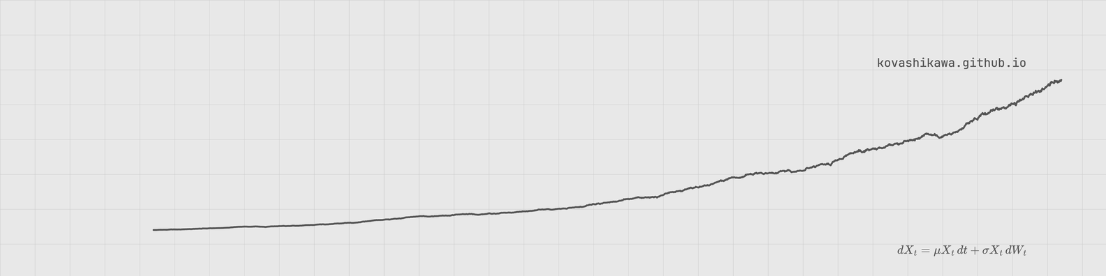
\[dX_t = \mu X_t\,dt + \sigma X_t\,dW_t\]
Geometric Brownian motion, the process Black-Scholes assumes for the
underlying. The curve is a single realized path: exponential drift, Brownian
noise. My preference is a quiet, monochrome plot in the same palette as this
blog, so that’s what this is.
A few decisions were deliberate.
A cover should be ambient
A LinkedIn banner is background. People come to the profile for the bio, the
experience, the work. So the cover gets three elements and nothing else: the
curve, a caption, and a URL. No axes, no ticks, no gridlines inside the plot.
If the values don’t matter, the scaffolding is noise. I kept the graph-paper
grid from this blog’s background, because it gives the curve a sense of place
without making it a chart.
Grey, not black, not blue
The data-viz literature converges on “grey plus one accent” for figures where
a specific element matters. But a cover is the opposite situation: nothing in
it should compete with the content below it. So the curve and caption are a
mid grey, the URL is a little darker for legibility, and there is zero hue.
Text on a cover dies
The placement that survived is symmetric: URL top-right, equation
bottom-right, both right-aligned to the same column. An equation is content
that describes the visual, so it sits on the visual like a caption. The URL
is a signature, so it sits in the corner like one. Two text elements, two
jobs, no overlap.
The crispness problem
Screenshot the HTML at 1x and a 2px curve is 2 physical pixels. It comes out
soft and aliased. The fix is a pipeline I now use every time I turn HTML into
an image:
Render in headless Chrome at 3x with --force-device-scale-factor=3,
giving a 4752x1188 master.
Downscale to the exact target with Pillow’s LANCZOS resampler.
sips -z is bilinear and softens edges; LANCZOS is the right filter.
Save as PNG, or JPEG around q=90 for a much smaller upload.
The text needed to be a touch bigger than I first wanted (17px, not 15px).
At 1584px wide, small glyphs are at the legibility floor.
The tool
All of it is one Python file now, so the next cover is one command:
kcover --seed 42 --out cover.png
It simulates a fresh path each run. Same equation, different realization,
which is the point. The seed pins a specific draw if you want to keep one.
It renders, downscales, and verifies the curve doesn’t collide with the
equation or the URL.
The cover is live on my profile.
If you see it in the wild, the curve you’re looking at is one sample path of
a stochastic differential equation. That’s the whole joke.
]]>{"name"=>nil, "avatar"=>"/assets/images/selfie-avatar.webp", "bio"=>"AI Engineer @ FUSE. Previously macro quant @ JGP. MIT MicroMasters. Washington, DC.", "location"=>"Washington DC", "email"=>nil, "links"=>[{"label"=>"Email", "icon"=>"fas fa-fw fa-envelope-square"}, {"label"=>"Website", "icon"=>"fas fa-fw fa-link"}, {"label"=>"Twitter", "icon"=>"fab fa-fw fa-twitter-square"}, {"label"=>"Facebook", "icon"=>"fab fa-fw fa-facebook-square"}, {"label"=>"GitHub", "icon"=>"fab fa-fw fa-github", "url"=>"https://github.com/kovashikawa"}, {"label"=>"LinkedIn", "icon"=>"fab fa-fw fa-linkedin", "url"=>"https://www.linkedin.com/in/rkovashikawa/"}]}MCP Grew Up Fast: From Experiment to Enterprise Trust Boundary2026-08-19T16:00:00+00:002026-08-19T16:00:00+00:00https://kovashikawa.com/ai/mcp-grew-up-fast“Why should you ever log into Salesforce again?”
Salesforce co-founder Parker Harris asked that out loud this spring, opening a product announcement most companies would never risk making about their own flagship product. By April 2026, Salesforce had shipped the part that made the question serious: a hosted, MCP connection any AI client can use to query a CRM in plain English, generally available to every Enterprise Edition org.
I spent the past few weeks building against exactly that surface. What struck me wasn’t the demo. It was realizing how recently the plumbing underneath it didn’t exist at all, and how fast it got built.
The 18 months that made this possible
MCP is barely two years old. Anthropic open-sourced it on November 25, 2024, after two engineers, David Soria Parra and Justin Spahr-Summers, had been building it since that July. What happened between then and Salesforce’s GA announcement is a compressed history of a protocol earning enterprise trust in real time, one hard problem at a time.
Can two systems even speak the same language? (Nov 2024 - Mar 2025)
MCP launched as a fairly narrow tool: JSON-RPC over stdio, mostly local processes talking to Claude Desktop. Useful for developers, not yet something a SaaS vendor would expose to the internet. That changed on March 26, 2025, when the spec’s second version added Streamable HTTP transport and, for the first time, a real OAuth 2.1-based authorization framework. The same day, OpenAI publicly committed to supporting MCP across its products, turning it from “Anthropic’s protocol” into the industry’s protocol.
Can you trust what’s on the other end? (Apr - Jun 2025)
Standardizing the wire format immediately exposed how little the security model had been stress-tested. In April 2025, Invariant Labs published a reproducible “tool poisoning attack,” the first serious public MCP exploit. It forced the issue. By June 18, the spec formally classified every MCP server as an OAuth 2.1 resource server under RFC 9728 (Protected Resource Metadata), meaning a server now had a standard, spec-defined way to declare who it trusted and what it would accept. Five days later, Salesforce anchored its Agentforce 3 platform around MCP interoperability and shipped its first servers.
Can an enterprise actually govern this? (Jun - Nov 2025)
A resource-server model is necessary but not sufficient for a Fortune 500 security review. Through the summer, the ecosystem built the governance layer the spec hadn’t yet: Cloudflare shipped MCP server portals, Auth0 published patterns for MCP-as-OAuth-resource-server, New Relic added MCP traffic observability. Then the November 25, 2025 spec, released on MCP’s first anniversary, formalized a lot of that community work directly into the standard: Client ID Metadata Documents replaced ad hoc dynamic client registration, an “Enterprise-Managed Authorization” extension let a company’s own identity provider broker trust instead of each vendor inventing its own, and PKCE went from recommended to mandatory.
Is this now just infrastructure? (Dec 2025 - Apr 2026)
Two weeks after that spec, on December 9, 2025, Anthropic donated MCP to the Linux Foundation’s new Agentic AI Foundation, co-founded with Block and OpenAI, backed by Google, Microsoft, AWS, Cloudflare, and Bloomberg. A protocol that started as one company’s open-source experiment was now nobody’s proprietary asset. Four months later, Salesforce’s Hosted MCP Servers went GA: OAuth 2.0 per user, scoped through an External Client App requesting mcp_api and refresh_token grants, fully managed on Salesforce’s own infrastructure. Seventeen months, roughly, from a two-person side project to the default way an AI agent gets audited, revocable, read-only access to a live enterprise CRM.
What that actually bought the people building on top of it
None of the above is abstract if you were the one wiring a client into it. Here’s the honest counterfactual, without walking through what I actually built: two years ago, an integration like this meant inventing your own answer, from scratch, to “how do I prove this credential can only read, only as this user, only against this one resource,” and then re-litigating that answer with every enterprise security team that asked. There was no shared vocabulary for it. Every vendor’s OAuth implementation was a slightly different bespoke argument.
What the spec’s maturation actually hands you now is that argument, pre-made. Audience-bound tokens are a defined behavior (RFC 8707), not a design choice you have to justify. Protected Resource Metadata means a server can advertise its own trust boundary instead of you documenting it out-of-band. Mandatory PKCE and a standardized insufficient-scope error path mean the failure modes a security reviewer asks about already have a spec-sanctioned answer. You’re not inventing a compliance story anymore. You’re citing one that a hundred other implementers already stress-tested.
That is, genuinely, the difference between a multi-quarter security review and something a small team can ship, get audited, and put in front of an enterprise admin in a reasonable window. Not because the engineering got easier. Because the trust model stopped being something each of us had to reinvent alone.
A personal note
I didn’t build any of the above. I’m one of a lot of engineers who happened to be building an integration during the window this protocol matured, and I got to feel the difference directly: a project that would have meant inventing a security model from scratch a year earlier instead meant adopting one that had already been through a public tool-poisoning exploit, a year of enterprise scrutiny, and formal standardization. That’s not a personal achievement. It’s what happens when a whole community, not just one vendor, spends eighteen months arguing about the right way to do this.
I’ll be talking about a related piece of this, deterministic evaluation and typed tool contracts for AI agents, at Google Search Central Live this year. Same underlying point: the hard problem in this space isn’t connecting to the data anymore. It’s trusting what comes back, and that’s only tractable now because the layer underneath got serious.
Two years, not a decade
A two-person open-source project became a Linux Foundation standard with mandatory security guarantees, adopted by every major AI lab, in under two years. That’s not normally how standards get made. Usually it takes a decade of committees. This one got there because a large number of people kept finding the gaps and fixing them in public, fast, under real pressure. Worth remembering next time an integration “just works” and it’s tempting to forget how much had to go right first.
Take Qwen3-1.7B, give it a set of BLS economic data tools, and distill it into a
specialist small enough to run on an M4 Mini. Ask it “what happened to food
prices since 2021?” and it should emit get_series(series_id="CUUR0000SAF1",
start="2021").
The pipeline: 205 hand-written seed questions over 82 economic concepts, 229
training examples, MLX LoRA, a 67MB adapter, six tools.
That part worked. Everything I initially believed about how well it worked was
wrong, in several separate ways, and finding each one required disproving the
previous one. The measurement was harder than the model. The fix, when it
finally came, was not a hyperparameter but a change to what the model was asked
to say.
Act 1: the number that wasn’t real
Round one looked clean. Train loss fell from 3.4 to 0.027. Fifteen held-out
examples, 87% accuracy. I fixed some data issues, retrained, got 93%. Base model
scored roughly zero. Ship it.
Then I ran a separate adversarial review of the pipeline, and none of it survived.
The held-out set was not held out. I had split the seeds before expanding
them, which sounds right. But the expander drew from shared pools (a list of
series IDs, a list of search terms) regardless of which split a seed belonged
to. So a training seed and a test seed could independently emit byte-identical
rows. 34% of my validation set appeared verbatim in training. Worse, the eval
file itself was stale: it was the first round’s holdout, and the second round’s
reshuffle had moved all 15 of those questions into training. The 93% was
measured on training data.
The metric was the easy half. “Accuracy” meant did it pick the right tool:
a 6-way classification. Whether the emitted call was actually correct was never
scored.
A ninth of the labels were wrong. Eleven series IDs named the wrong concept.
CUUR0000SETG01 was mapped to “energy”; the BLS catalog calls it airline
fares. CUUR0000SAH1 was “housing” but means shelter; CUUR0000SAM1 was
“medical care” but means medical care commodities. Four IDs (SAR1, SAC1,
SAS1, SEHA01) do not exist in any BLS catalog at all. I had invented them by
pattern-matching the real ones.
The lesson I’d draw is not “be careful.” It’s that every one of these bugs
pushed the number up. Nobody investigates a pleasant surprise as hard as a
disappointing one, and that asymmetry is the whole problem.
Act 2: testing the impossible
Fixing the leak exposed a deeper design error.
The split held out whole concepts. If “medical care” appeared only in the test
set, the model was being asked to produce CUUR0000SAM having never once seen
that mapping. Four of eleven scored items were unanswerable by construction.
This is a lookup task. "medical care" → CUUR0000SAM cannot be derived from
first principles; it can only be recalled. So the split should hold out
phrasings, not concepts:
Every concept contributes at least one phrasing to training
Remaining phrasings go to val/test
The build fails if any concept is held out entirely
I rewrote the seed data as concept tables (82 concepts, each with 2+ distinct
phrasings) and added build-time assertions: every series ID must exist in the
bundled 8,103-row catalog, no example may appear in two splits, no concept may be
missing from train. Assertions, not intentions. Two of them have fired on me
since.
Act 3: the discovery
With clean data I swept checkpoints from 100 to 1400 iterations, planning to pick
the lowest validation loss like every tutorial says.
Val loss bottomed at iteration 250 and rose steadily afterward. Textbook
overfitting. But I was also scoring actual tool-call accuracy, and the two
disagreed violently:
iter
val loss
exact match
200
0.135 (min)
37.2%
400
0.135
65.1%
600
0.147
90.7%
800
0.156
81.4%
1000
0.169
88.4%
1400
0.169
74.4%
Stopping at the val-loss minimum would have shipped a 37% model instead of a 91%
one. I wrote this up as a finding: val loss is a trap for structured-output
tasks. Cross-entropy punishes a confidently-wrong series ID exactly as hard as
gibberish, while a task evaluator sees a near-miss. I had citations lined up.
It was a config bug.
Act 4: disproving my own finding
Before publishing I checked one number I had never looked at: the ratio of
completion length to prompt length.
mean prompt tokens     : 134
mean completion tokens :  19
generation ratio       : 0.141
Every training row carried a ~120-token system prompt, byte-identical across the
dataset, and a ~19-token tool call. And I was training with prompt loss
unmasked.
87.7% of every gradient was the model re-predicting a fixed preamble.
That explains all of it. Train loss of 0.027 was never impressive: most of it
was copying a constant. And validation loss was ~88% a measurement of preamble
reproduction, which is uncorrelated with whether the tool call is right. The two
curves weren’t in tension for any deep reason. One of them was mostly noise.
This is documented. Huerta-Enochian and Ko (2024) found a statistically
significant effect of prompt-loss weight specifically for short-completion data,
and Vaughn’s walkthrough of the same phenomenon on a multiple-choice dataset
(generation ratio 0.01) reports that stopping at the full-sequence val-loss
minimum yields 53% accuracy while completion loss is still falling. I reproduced
a known failure mode and mistook it for a discovery.
So I masked the prompt and reran. Prediction: val loss should re-couple with
accuracy.
iter
val loss (masked)
exact match
200
0.046
62.8%
400
0.028
86.0%
600
0.027 (min)
90.7%
800
0.028
90.7%
unmasked
masked
pick by val-loss minimum
37.2%
86.8%
best checkpoint available
90.7%
88.4%
penalty for trusting val loss
~50 pts
1.6 pts
The trap was self-inflicted. Mask the prompt and standard practice works fine.
Switching to chat-format data to enable masking fixed two other things I had been
carrying without noticing: Qwen3’s chat template emits an empty
<think></think> block, which is the actual mechanism for non-thinking mode;
I had been asking for it in English in the system prompt, which is not the same
thing. It also removed a stray leading space before every tool call that made the
training target tokenize differently from anything an inference path would
produce.
Act 5: the thing that actually mattered
Here is the result I should have led with, and it is the least exciting one.
I had been quoting 90.7%. To check reproducibility I retrained with three
different random seeds, changing nothing else:
seed
exact match
0
76.7%
1
81.4%
2
90.7%
3
88.4%
Mean 84.3%, standard deviation 6.4 points, range 14 points.
90.7% was not the result. It was the best of four draws. At this dataset size a
single run tells you almost nothing, and every comparison I had made (including
one where I concluded a data fix had caused a 14-point regression) was inside
the noise. That “regression” was seed 0 landing at the bottom of the
distribution. I nearly reverted a correct fix because of it.
After the config fixes (prompt masking, all 28 layers instead of 16, rank 16,
cosine schedule with warmup), across three seeds:
Mean 88.4%, standard deviation 4.0. Better mean, tighter spread, and a
validation signal that now points the right way.
An interlude on measurement
Small-data fine-tuning has terrible measurement ergonomics. Nearly every mistake
in this project was a measurement mistake, not a modelling one:
A test set that wasn’t held out
A metric that scored the easy half of the task
Labels that were confidently wrong
A test that asked for things never taught
A loss dominated by a constant
Single-run numbers with 14 points of spread
Gold labels in a stale format, scoring correct answers as wrong
The model was never the hard part. None of these were visible from the loss
curve. The first six all made the number look better than reality, which is why
they all survived. The seventh made it look catastrophically worse, and I nearly
abandoned a good idea because of it.
Act 6: the part hyperparameters couldn’t fix
The config work moved 84% to 88% and stalled. Every remaining failure was sibling
confusion between near-identical codes: CUUR0000SAF11 (food at home) vs
CUUR0000SAF1 (food), CUUR0000SAM (medical care) vs CUUR0000SEMD (hospital
services). Those aren’t bugs. That’s what memorizing a codebook into weights looks
like at the margin, and no learning rate fixes it.
I was training a 1.7B model to recall 13-character opaque strings where a
one-character slip silently fetches a different economic series. Lookup tables
don’t belong in weights. So before writing that as an opinion, I measured it.
Measuring the alternative
First a correction to my own framing. I had been saying the catalog has 8,103
series, so memorization covers 0.4% of it. That number is misleading. The catalog
is really 400 distinct items repeated across ~20 area and seasonal-adjustment
combinations. “Housing” matches 120 titles because the same concept appears for
US city average, Northeast, New England, Chicago, seasonally adjusted and not.
Constrained to the namespace every one of my seeds actually uses (US city
average, not seasonally adjusted): the corpus is 400 rows, and the item name is
a unique key. That reframes the problem: not 8,103 codes to memorize, but 400
well-named items to look up. Still 11x more than the 35 I could afford to
teach, but a completely different kind of problem.
So I built a ~30-line BM25 index over those 400 item names and measured recall of
the correct series ID on the same 43 held-out questions:
query
recall@1
recall@5
oracle (the gold item’s own name)
100%
100%
the raw user question, no model at all
84.4%
93.8%
The first row says the retriever has no ceiling problem: given a decent query it
is perfect. The second row is the uncomfortable one. Throwing the user’s raw
question at BM25 (no model, no training, no GPU, no adapter) retrieves the
correct series 84.4% of the time, against 88.4% for the fine-tuned model. Those
are within noise of each other.
A week of distillation is currently tied with a text search over 400 strings.
And the two questions raw BM25 misses are precisely the two my fine-tuned model
gets wrong:
want  Medical care                          from "Show me healthcare CPI..."
want  Owners' equivalent rent of primary…   from "What did OER do between…"
Both are vocabulary gaps: “healthcare” and “OER” don’t appear in the official
item names. So the obvious move is to have the model rewrite the user’s words
into catalog vocabulary and let retrieval do the lookup. Much easier than
emitting a 13-character code from memory, and it generalizes to all 400 items.
I tested that too, and it does not work yet:
query source
recall@1
recall@5
oracle (gold item name)
100%
100%
raw question, no model at all
84.4%
93.8%
base Qwen3-1.7B rewrites the question
75.0%
84.4%
my fine-tuned model rewrites it
62.5%
71.9%
Every model in the chain makes retrieval worse. The base model degrades good
queries. Asked about “tuition, other school fees, and childcare”, which is
verbatim the official item name, it helpfully rewrites it to “Education
expenses”. Asked about OER it expands the acronym to “Educational Resources
(OER)”, which is a real term from a different field entirely.
My fine-tuned model is worse still, and the reason is the interesting part.
Asked for a search phrase, it emits series IDs:
"What did education and communication prices do…"  →  CUUR0000SAEDECU01
"Show me tuition and childcare CPI…"               →  CUUR0000SEEB
"Show me healthcare CPI…"                          →  search_phrase:CUUR0000SEMD Healthcare
It has specialized so hard on emitting codes that it can no longer paraphrase.
Note the second line: CUUR0000SEEB is the correct answer. The model knows the
mapping. It just can’t express it in a form the retriever can use, because the
index is over item names and it only speaks in IDs.
That is a useful negative result. It means retrieval cannot be bolted onto this
adapter: the memorization fine-tune destroyed the exact capability retrieval
depends on. The two-step system has to be trained from base, on traces that
include the search step, and Anthropic’s caution about small models and query
formulation is now something I’ve measured on my own data rather than quoted.
Act 7: the fix was the output format
The agent ecosystem has converged on retrieval for a structurally identical
problem one level up. Hermes Agent, mcp-sieve, and various tool-router plugins
all replace “load every tool schema” with a search → describe → call
bridge. Anthropic’s MCP evaluations show accuracy improving when tools are
deferred rather than preloaded (49% → 74% on Opus 4) because large catalogs
cause decision paralysis.
Their bottleneck is too many tools. Mine was 400 values in one argument slot. So
I was about to build the two-step system, and then noticed I could get most of
the benefit by changing one thing: what the model is asked to emit.
get_series(series_id="CUUR0000SAF11") → get_series(item="Food at home")
The model names the item; forty lines of code resolve the name to an ID. This
works only because of the 400-item finding above: item name is a unique key
in that namespace, so the resolution is deterministic, not a guess.
Why it helps is the same reason the failures were what they were. SAF11 vs
SAF1 is a one-character discrimination. “Food at home” vs “Food” is a
semantic one, which is the kind of distinction a language model is actually built
to make. And a name fails loudly: resolve_item returns None for something
it can’t place, where one wrong character in a code silently fetches a different
series and returns plausible numbers.
Five seeds, same 43 held-out phrasings:
target format
exact
sd
get_series(series_id="CUUR0000SAF11")
88.8%
3.0
get_series(item="Food at home")
92.1%
1.3
+ hierarchy-aware resolver
94.4%
1.3
+5.6 points, t = 3.8, p ≈ 0.005, and seed variance more than halved.
Exact match on 43 held-out phrasings
Same held-out set throughout. The originally reported 93% is not shown — it was measured on training data. The final row (+alias) is the same model with the resolver alias table; see Act 8 on why it is not the headline number.
base Qwen3-1.7Bno fine-tuning
9.3%
V2, honestly measuredthe real starting point
13.3%
BM25 over 400 itemsno model at all
84.4%
+ prompt masking, r16config fixes
88.8% ±3.0
+ item-name targetsoutput format
92.1% ±1.3
+ hierarchy resolvercurrent
94.4% ±1.3
+ alias table†see Act 8
96.7% ±1.3
0%25%50%75%100%
fine-tuned, successive fixesbaseline, no fine-tuning±1 sd across 5 seeds
Table view
Stage
Exact
sd
Kind
base Qwen3-1.7B
9.3%
—
baseline
V2, honestly measured
13.3%
—
fine-tuned
BM25 over 400 items, no model
84.4%
—
baseline
+ prompt masking, all layers, rank 16
88.8%
±3.0
fine-tuned
+ item-name targets
92.1%
±1.3
fine-tuned
+ hierarchy-aware resolver
94.4%
±1.3
fine-tuned
+ alias table †
96.7%
±1.3
fine-tuned
Held-out phrasings absent from training, every referenced concept present.
Fine-tuned rows are means over five training seeds; the three single-measurement
rows carry no error bar rather than an invented one.
The hierarchy rule is small: when a bare term is a whole-word prefix of several
catalog entries, prefer the general one: “tobacco prices” means Tobacco and
smoking products, not Tobacco products other than cigarettes.
The only remaining failures at this point are “healthcare” → Medical care and
“OER” → Owners’ equivalent rent. Both are vocabulary gaps the resolver cannot
bridge without knowing which official term the user meant. The alias table was
the obvious fix, and the obvious problem: both failures are visible from
reading the test set.
And the first run of this experiment reported 23.3%. A catastrophic
regression that would have killed the idea. It was a scoring bug: the held-out
file still stored raw series_id while the model now emitted item names, so
every correct answer scored wrong. I caught it because 10 of 43 passed, and
exactly 10 test items have no series ID. Gold is now rendered by the same
function that builds training targets, so the two cannot drift again.
That’s the second phantom regression in this project. Both times the number said
“your change broke it” and both times the number was the broken thing.
A note on the “100% accuracy” claims circulating in the tool-router ecosystem: I
read them. One is 10 out of 10 test cases. Another is 100% on synthetic
validation data generated the same way as its training data. Both are the same
species of number as my original 93%. Copy the architecture; don’t quote the
benchmarks.
Act 8: the alias table
The two failures were “healthcare” → Medical care and “OER” → Owners’
equivalent rent. I said I was leaving them in. Then I shipped the alias table.
The number, same five adapters, model untouched:
exact
sd
fine-tuned, item names
94.4%
1.3
+ resolver alias table
96.7%
1.3
The accounting matters. There are roughly 50 aliases in the table: groceries,
gas, core CPI, airfare, public transport. Against this eval they move nothing;
its 43 questions don’t use that vocabulary. The entire +2.3pp is healthcare.
That alias was added knowing it was one of my two held-out failures.
Which makes it contaminated by the definition this post uses. I reported 94.4%
as the model’s number and put the alias row in a footnote.
The tension is that healthcare is simultaneously the most obvious synonym a
real user types and one of my two known test failures. Omitting it from a
user-facing resolver to protect a benchmark would be absurd. So no option was
both maximally useful and maximally clean.
What that means more broadly: once you’ve read your test failures, you can’t
un-read them. The honest options narrow permanently. The stricter path was to
build the alias table from general domain vocabulary, validate it on the val
split, and leave test untouched. I didn’t do that. I reported both numbers and
disclosed which one was contaminated. Honest, but not maximally rigorous, and
the distinction is real.
OER is still failing. The model emits item="Education and communication", a
hallucination the resolver cannot repair. That is a model error, not a vocabulary
gap, and an alias does nothing for it.
One item remains genuinely open: enumerate all 400 names in context and let the
model select from a visible list rather than recall from memory. At 2,274 tokens
it fits, and it removes the lookup problem entirely for anything the model can
phrase correctly.
What I would do differently
Check your generation ratio before anything else. If completions are short
relative to prompts, mask the prompt. Otherwise your loss is mostly measuring
whether the model can copy a constant, and any conclusion you draw from that
curve is suspect.
Report a distribution, not a run. Three seeds minimum, five if the difference
matters. At n=43 with 6 points of seed variance, a single number is close to
meaningless. If you only rerun the results you dislike, you will systematically
publish your luckiest draws.
Write assertions, not intentions. “The splits are disjoint” is a claim. A
build that fails when they aren’t is a guarantee. Mine now refuses to run if any
series ID is absent from the catalog, if any example appears twice, if any
concept is missing from training, or if any label mentions dates its question
doesn’t.
Split by what the model must actually generalize over. For a lookup task,
hold out phrasings. Holding out concepts measures the impossible.
Ask what you’re making the model say, not just how you’re training it. The
single largest improvement in this project (+5.6 points, variance halved) came
from changing the output format from an opaque ID to a name, not from any
hyperparameter. Errors that are one character apart are hard for a language
model; errors that are semantically apart are easy. And a name can fail loudly
where a code fails silently.
Measure the dumb baseline first. Thirty lines of BM25 over 400 strings scores
84.4% here. I was five days in before I knew that, and for all five of those days
I was comparing my results against nothing. If the baseline had come out ahead,
the right answer would have been to delete the model.
Be most suspicious of results you like. Six of the seven bugs above inflated
my numbers. That is not coincidence: unpleasant surprises get debugged, pleasant
ones get published.
Once you’ve read your test failures, you can’t un-read them. The honest
options narrow. If you’re building something that touches items you know failed,
validate it on val, not test. I didn’t; I reported both numbers and disclosed the
contamination. Honest, not maximally rigorous. The difference matters.
Results
43 held-out phrasings, none seen in training, every referenced concept present.
Mean over five training seeds, +/- one standard deviation across seeds:
tool
entity
exact
base Qwen3-1.7B
72.1%
9.3%
9.3%
fine-tuned, emitting series IDs
99.1% +/- 1.3
89.8% +/- 2.1
88.8% +/- 3.0
fine-tuned, emitting item names
99.1% +/- 1.3
94.4% +/- 1.3
94.4% +/- 1.3
+ resolver alias table
99.1% +/- 1.3
96.7% +/- 1.3
96.7% +/- 1.3 †
raw BM25 over 400 items, no model
–
–
84.4%
tool — correct function chosen, out of six
entity — plus the load-bearing argument (series ID / query / survey)
exact — every argument identical
† Same five adapters, model untouched. The entire +2.3pp is the
healthcare alias, added knowing it was a held-out failure. See Act 8.
A 67MB adapter on an M4 Mini, for the 35 concepts it was taught. I want to
resist rounding that 99.1% to “100%”; four of five seeds hit 43/43 and the
temptation to quote the clean number is exactly the reflex this whole exercise
was about.
Worth stating the cost honestly: the config fix took the adapter from 19MB to
67MB, because it raised LoRA rank from 8 to 16 and adapted all 28 transformer
blocks instead of the last 16. So +4.5 points of exact match came with 3.5x the
adapter size. I did not sweep that tradeoff; rank 8 across all layers might get
most of the gain at half the size, and I have not checked.
The third row is there because a serious writeup should include the baseline
that embarrasses it.
One last operational note, learned the annoying way: I ran an evaluation
concurrently with a training job on the same GPU and got different numbers for
identical weights. Not non-determinism (two isolated runs are byte-identical),
but under memory pressure MLX returned different results rather than simply
running slower. I nearly wrote up a phantom regression from it. Score on a quiet
machine.
Huerta-Enochian, M. & Ko, S. Y. (2024). “Instruction Fine-Tuning: Does Prompt
Loss Matter?” EMNLP 2024. arXiv:2401.13586
Guo, H., Dennis, S., Patil, R., & Shabahang, K. (2026). “When Mean CE Fails:
Median CE Can Better Track Language Model Quality.”
arXiv:2605.24667. Finds mean cross-entropy
rising while held-out accuracy stays near peak, in Qwen2.5-1.5B SFT.
Apicella, A., Isgrò, F., Pollastro, A., & Prevete, R. (2026). “Don’t stop me
now: Rethinking Validation Criteria for Model Parameter Selection.”
arXiv:2602.22107. Finds early stopping on
validation accuracy performs worst for neural classifiers, favouring
loss-based criteria. Worth reading against this post: their objection is to
early stopping specifically, and they find post-hoc selection across all epochs
comparable to loss-based selection.
Chatterjee, A., Renduchintala, H. S. V. N. S. K., Bhatia, S., & Chakraborty, T.
(2025). “On the Effect of Instruction Tuning Loss on Generalization.”
arXiv:2507.07817. Finds fully masking
prompt tokens is rarely optimal either; a low-to-moderate prompt weight usually
beats both extremes.
Vaughn, D. (2024). “To Mask or Not to Mask: The Effect of Prompt Tokens on
Instruction Tuning.” Towards Data Science.
]]>{"name"=>nil, "avatar"=>"/assets/images/selfie-avatar.webp", "bio"=>"AI Engineer @ FUSE. Previously macro quant @ JGP. MIT MicroMasters. Washington, DC.", "location"=>"Washington DC", "email"=>nil, "links"=>[{"label"=>"Email", "icon"=>"fas fa-fw fa-envelope-square"}, {"label"=>"Website", "icon"=>"fas fa-fw fa-link"}, {"label"=>"Twitter", "icon"=>"fab fa-fw fa-twitter-square"}, {"label"=>"Facebook", "icon"=>"fab fa-fw fa-facebook-square"}, {"label"=>"GitHub", "icon"=>"fab fa-fw fa-github", "url"=>"https://github.com/kovashikawa"}, {"label"=>"LinkedIn", "icon"=>"fab fa-fw fa-linkedin", "url"=>"https://www.linkedin.com/in/rkovashikawa/"}]}Winning the Google Cloud AI Hackathon: Building Multimodal Medical Annotation at Scale2026-01-09T00:00:00+00:002026-01-09T00:00:00+00:00https://kovashikawa.com/projects/ai/google-cloud-ai-hackathon-winnerOverview
Last month, I participated in the Google Cloud AI Hackathon, a fast-paced competition focused on building applied AI systems with real deployment constraints.
Our project, MedAnnotator, was selected as one of the winning teams.
The official announcement is available here:
👉 https://opendatascience.com/highlighting-the-winners-of-the-december-2025-google-cloud-ai-hackathon/
The problem we addressed is well known in medical AI:
Medical image annotation is expensive, slow, inconsistent, and difficult to scale, yet it remains a critical dependency for clinical workflows, research, and model development.
Our goal was to design a system that prioritizes correctness, structure, and deployability, rather than novelty.
Problem Definition
We identified three core bottlenecks in existing medical image annotation workflows:
Limited scalability: Annotation relies heavily on expert time, which does not scale with data volume.
High label variance: Inter-annotator disagreement introduces noise and reduces downstream model reliability.
Unstructured outputs: Free-text annotations are difficult to validate, audit, or integrate into pipelines.
The system was designed to generate structured, reviewable annotations from medical images while explicitly supporting human oversight.
System Architecture
1. Two-Tier Model Design
Rather than relying on a single model, we decomposed the task:
MedGemma: Responsible for domain-specific medical image understanding. This model handled image-level reasoning and feature extraction.
Gemini (API): Used for validation, reasoning over MedGemma outputs, and producing structured, schema-compliant annotations.
This separation reduced coupling, improved iteration speed, and made failure modes easier to reason about.
2. Structured Outputs as a First-Class Constraint
All annotations were generated using predefined schemas.
We deliberately avoided free-form text.
This experience reinforced several principles that consistently hold in applied AI:
System design often matters more than model size.
Structured outputs outperform clever prompts in production settings.
Human-in-the-loop workflows remain essential in high-stakes domains.
Deployment constraints improve, rather than limit, design quality.
Future Extensions
The prototype can be extended in several directions:
Batch annotation pipelines for large-scale datasets
Integration with PACS or clinical data systems
Active learning loops using corrected annotations
Quantitative evaluation tooling for annotation quality and drift
If you are working on applied multimodal systems, especially in healthcare, I am always open to technical discussions.
Thanks to my teammates, ODSC, and Google Cloud for running a technically rigorous and well-executed hackathon.
]]>{"name"=>nil, "avatar"=>"/assets/images/selfie-avatar.webp", "bio"=>"AI Engineer @ FUSE. Previously macro quant @ JGP. MIT MicroMasters. Washington, DC.", "location"=>"Washington DC", "email"=>nil, "links"=>[{"label"=>"Email", "icon"=>"fas fa-fw fa-envelope-square"}, {"label"=>"Website", "icon"=>"fas fa-fw fa-link"}, {"label"=>"Twitter", "icon"=>"fab fa-fw fa-twitter-square"}, {"label"=>"Facebook", "icon"=>"fab fa-fw fa-facebook-square"}, {"label"=>"GitHub", "icon"=>"fab fa-fw fa-github", "url"=>"https://github.com/kovashikawa"}, {"label"=>"LinkedIn", "icon"=>"fab fa-fw fa-linkedin", "url"=>"https://www.linkedin.com/in/rkovashikawa/"}]}Analysing the impact of AI jobs at World Bank DataDive 20252025-12-08T00:00:00+00:002025-12-08T00:00:00+00:00https://kovashikawa.com/ai/data-science/labor/worldbank-datadive-hackathonBuilding JobsLens AI at World Bank DataDive 2025
Last week, I participated in the World Bank DataDive 2025, a 8-hour hackathon focused on extracting insights from global labor market data. Our team of five—Maryam Shahbaz Ali, Paul Suhwan Lee, Stevens Cadet, Yingquan Li, and myself—tackled Challenge 8: Digital/AI Job Demand & Supply Analysis.
TL;DR: We built JobsLens AI, an interactive Gradio dashboard that visualizes AI job market trends across countries, identifies skills gaps, and forecasts future demand.
The Challenge
The World Bank wanted to understand where digital and AI job opportunities are rising or lagging across countries, industries, and skill types. The goal was to help policymakers identify:
Countries with high AI job demand but low skilled workforce supply (skills gaps)
Emerging markets with growing AI sectors
Trends in AI talent concentration and investment
The Data
We worked with two primary datasets:
Stanford HAI AI Index 2025 (528 observations, 232 columns)
World Bank Global Labor Database (154 countries, cross-sectional)
Employment rates by sector and education level
Labor force participation, unemployment rates
Demographics and population statistics
Technical Approach
Data Integration Challenge
The fundamental problem was joining cross-sectional predictors (World Bank) with panel outcomes (HAI):
HAI: Multiple years per country (2017-2024)
World Bank: Single observation per country
We used a many-to-one merge, assuming labor market characteristics remain relatively stable over time.
Dashboard Development
Built with Gradio 4.0 and Plotly, the dashboard features 5 interactive tabs:
🌍 Global Overview: Choropleth map showing supply-demand gaps
📊 Country Comparison: Multi-country trend analysis (default: Brazil, Argentina, USA, Japan)
🏆 Rankings: Top countries by AI job demand, skills supply, investment, startups
🔮 Forecasts: 2024-2025 projections built with a minimalist linear trend baseline after richer models proved unreliable under the time and data constraints
🔬 Country Deep Dive: Detailed statistics for individual countries
Deployment
We deployed to Hugging Face Spaces for free hosting:
Forecasting was the toughest part: with only a few hours to wrangle unfamiliar data, every richer model we tried failed to be accurate, robust, or remotely reliable. I fell back to a simplistic linear trend model so the projections stayed within clearly understood limitations. Even so, the exploratory dashboard successfully visualizes historical trends and provides policymakers with actionable insights on global AI skills gaps.
Future Improvements
If I were to continue this project:
Use “All” subsample instead of “Urban” to get 24/24 features
Time-series models: ARIMA or exponential smoothing might outperform ML on small data
External data: Add OECD education stats, GitHub commit data by country
Sector analysis: Break down AI jobs by industry (healthcare, finance, etc.)
Interactive filtering: Let users select custom country groups and metrics
Explore AI job trends for 66 countries, compare Brazil vs. USA, or dive into Switzerland’s AI ecosystem. The dashboard is free and requires no login.
Hackathon: World Bank DataDive 2025Team: JobsLens AIDuration: 8 hoursTech: Python, Gradio, Plotly, scikit-learn, Hugging Face Spaces
]]>{"name"=>nil, "avatar"=>"/assets/images/selfie-avatar.webp", "bio"=>"AI Engineer @ FUSE. Previously macro quant @ JGP. MIT MicroMasters. Washington, DC.", "location"=>"Washington DC", "email"=>nil, "links"=>[{"label"=>"Email", "icon"=>"fas fa-fw fa-envelope-square"}, {"label"=>"Website", "icon"=>"fas fa-fw fa-link"}, {"label"=>"Twitter", "icon"=>"fab fa-fw fa-twitter-square"}, {"label"=>"Facebook", "icon"=>"fab fa-fw fa-facebook-square"}, {"label"=>"GitHub", "icon"=>"fab fa-fw fa-github", "url"=>"https://github.com/kovashikawa"}, {"label"=>"LinkedIn", "icon"=>"fab fa-fw fa-linkedin", "url"=>"https://www.linkedin.com/in/rkovashikawa/"}]}MCP: Inside the Data Layer and the Choice of JSON-RPC 2.02025-10-15T21:18:00+00:002026-08-26T00:00:00+00:00https://kovashikawa.com/ai/mcp-notesWhat MCP is for
The Model Context Protocol (MCP) is an open specification, released by Anthropic in November 2024, that defines a single interface between AI models and external systems. A client (an agent) and a server (a tool, database, or API wrapper) exchange protocol versions and capabilities at connect time, then communicate through four primitives: tools, resources, prompts, and notifications. That structure is JSON-RPC 2.0.
Why JSON-RPC 2.0 over plain JSON
Plain JSON over HTTP gives you a body and a status code. Nothing defines the method name, nothing links a response to the request that produced it, and there is no agreed error shape.
JSON-RPC 2.0 fixes each of those. Every message carries jsonrpc: "2.0", a method, params, and an id that correlates responses with requests. A server can reply asynchronously and out of order, and can issue its own calls back to the client, which is what lets a long-running tool stream progress while another call completes.
Notifications are JSON-RPC messages without an id; the sender expects no reply. MCP uses them for progress and log messages. Batch requests send several calls in one array and receive the responses together. Both map directly to agent workloads, where a model issues several tool calls in a row.
The transports: stdio and Streamable HTTP
JSON-RPC defines message framing independently of transport, so the same logical message moves over different channels. MCP specifies two.
stdio: the client spawns the server as a child process and exchanges JSON-RPC messages over standard input and output. No HTTP stack, no serialization boundary. The default for local servers.
Streamable HTTP: a single HTTP connection the server can stream incremental responses over. It replaced the earlier HTTP + SSE transport, which the spec deprecated in March 2025. The server can push updates over the same connection, which matters for tools that run for seconds rather than milliseconds.
The transport changes the deployment model, not the messages. The same tools/call payload works over stdio locally and over Streamable HTTP remotely.
The data layer: tools, resources, and capability negotiation
The data layer defines what the messages can carry. At connect time, client and server exchange protocol versions and capabilities. The server then publishes its surface:
tools: functions the model can call, each described by name, description, and an input JSON Schema
resources: readable data surfaces, identified by URI and MIME type
prompts: reusable prompt templates the client can request
notifications: server-initiated events the client can register for
This is what makes the protocol composable. A model never needs per-API glue: the schema of every tool arrives during the handshake, so a client can construct valid arguments and validate the result without knowing anything about the underlying service.
Errors are part of the contract
JSON-RPC 2.0 reserves a base set of error codes, and MCP adds its own on top. Every failed call returns an object with code, message, and optional diagnostic data. When an agent chains several tool calls, a typed error lets it branch on the failure mode instead of guessing from a bare HTTP status.
]]>{"name"=>nil, "avatar"=>"/assets/images/selfie-avatar.webp", "bio"=>"AI Engineer @ FUSE. Previously macro quant @ JGP. MIT MicroMasters. Washington, DC.", "location"=>"Washington DC", "email"=>nil, "links"=>[{"label"=>"Email", "icon"=>"fas fa-fw fa-envelope-square"}, {"label"=>"Website", "icon"=>"fas fa-fw fa-link"}, {"label"=>"Twitter", "icon"=>"fab fa-fw fa-twitter-square"}, {"label"=>"Facebook", "icon"=>"fab fa-fw fa-facebook-square"}, {"label"=>"GitHub", "icon"=>"fab fa-fw fa-github", "url"=>"https://github.com/kovashikawa"}, {"label"=>"LinkedIn", "icon"=>"fab fa-fw fa-linkedin", "url"=>"https://www.linkedin.com/in/rkovashikawa/"}]}Architects, Anthills, and AI: A Nobel Prize’s Lesson on Scientific Progress2025-10-09T00:00:00+00:002025-10-09T00:00:00+00:00https://kovashikawa.com/ai/architecs-anthill-aiThe 2025 Nobel Prize in Chemistry has been awarded to Susumu Kitagawa, Richard Robson, and Omar M. Yaghi for their creation of an entirely new class of materials: metal-organic frameworks (MOFs)[1].
These remarkable materials can be thought of as molecular sponges or programmable crystals. Built from metal ions and organic linkers, their defining feature is a vast internal porosity, allowing just a few grams to have a surface area the size of a football pitch. This unique property has unlocked potential solutions to some of humanity’s biggest challenges, from capturing carbon dioxide and harvesting water from desert air to filtering pollutants and delivering drugs.
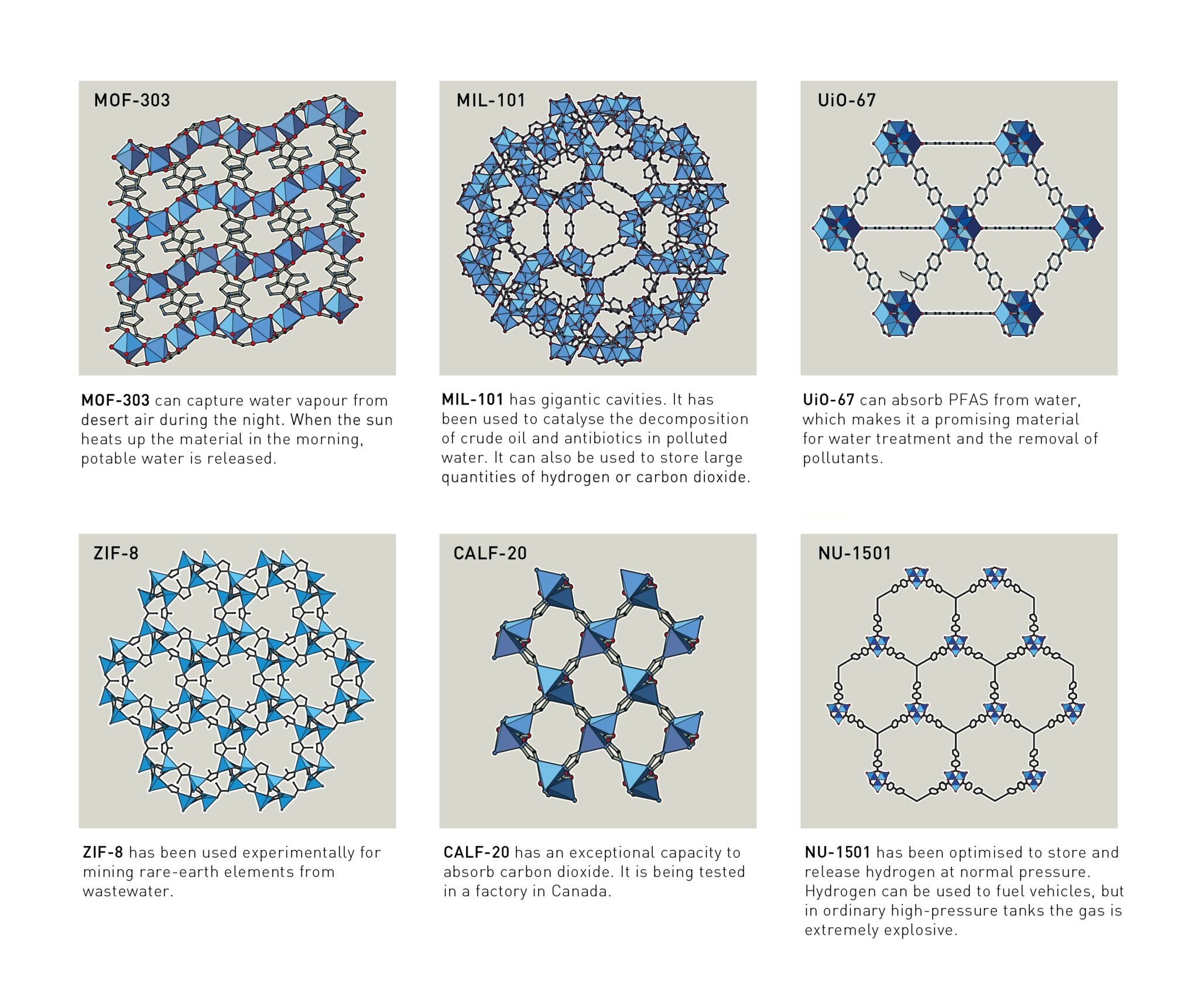
Figure: The versatility of MOFs is staggering. Different frameworks are tailored for specific tasks, such as capturing water from air (MOF-303), storing hydrogen fuel (MIL-101), removing PFAS pollutants from water (UiO-67), and absorbing industrial CO₂ emissions (CALF-20), showcasing the breadth of research built upon the laureates’ foundational work.
The laureates’ journey is a story of visionary science. It began with Richard Robson’s foundational idea to build large, ordered networks. Building on this, Susumu Kitagawa developed the first stable, functional MOFs and crucially envisioned them as flexible structures that could “breathe.” Omar M. Yaghi then perfected the field by demonstrating a “Lego-like” approach to their creation, allowing chemists to rationally design frameworks with tailored properties, including his iconic and exceptionally spacious MOF-5.
This tale of three pioneers seems like a classic case of the “Newtonian” view of science—that progress is driven by a few brilliant giants who provide the shoulders for others to stand on. However, the story of MOFs also powerfully illustrates a competing idea: the Ortega hypothesis[2]. This theory suggests that major breakthroughs don’t happen in a vacuum. Instead, they arise from the slow, cumulative, and often anonymous contributions of a great number of working scientists.
This is where Susumu Kitagawa’s personal motto—to find “the usefulness of useless”—becomes profoundly insightful. Science is filled with countless small experiments and niche discoveries that seem purposeless in isolation. The Ortega hypothesis argues that progress depends on this vast, unglamorous foundation of “useless” knowledge. It’s an ecosystem of modest findings that a few brilliant minds can eventually synthesize into a revolutionary concept. The laureates themselves were building on decades of fundamental chemistry. Kitagawa’s philosophy wasn’t just a personal quirk; it was an acknowledgment of the very nature of scientific progress.
We see this process in action right now. Today, labs across the globe are using the MOF toolkit to design countless specialized frameworks [3]. Each team works on a narrow problem—a single pollutant, a specific gas, a unique catalyst. Each contribution is a small, vital step forward, an anthill of progress built upon the architectural plans the laureates drew.
The laureates’ work defined a design space so vast it became a big data problem, which global research has populated and AI can now analyze.
Instead of relying on slow physical synthesis, AI models computationally screen millions of potential MOFs to pinpoint the most effective candidates for tasks like carbon capture. This is the new paradigm for discovery: human genius creates the field, collective effort generates the data, and AI provides the scaling engine to find the solutions within.